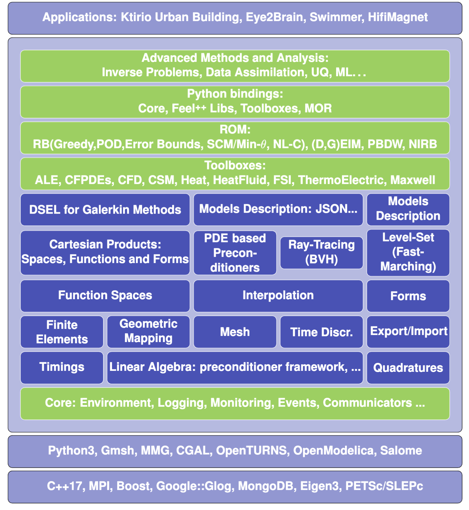
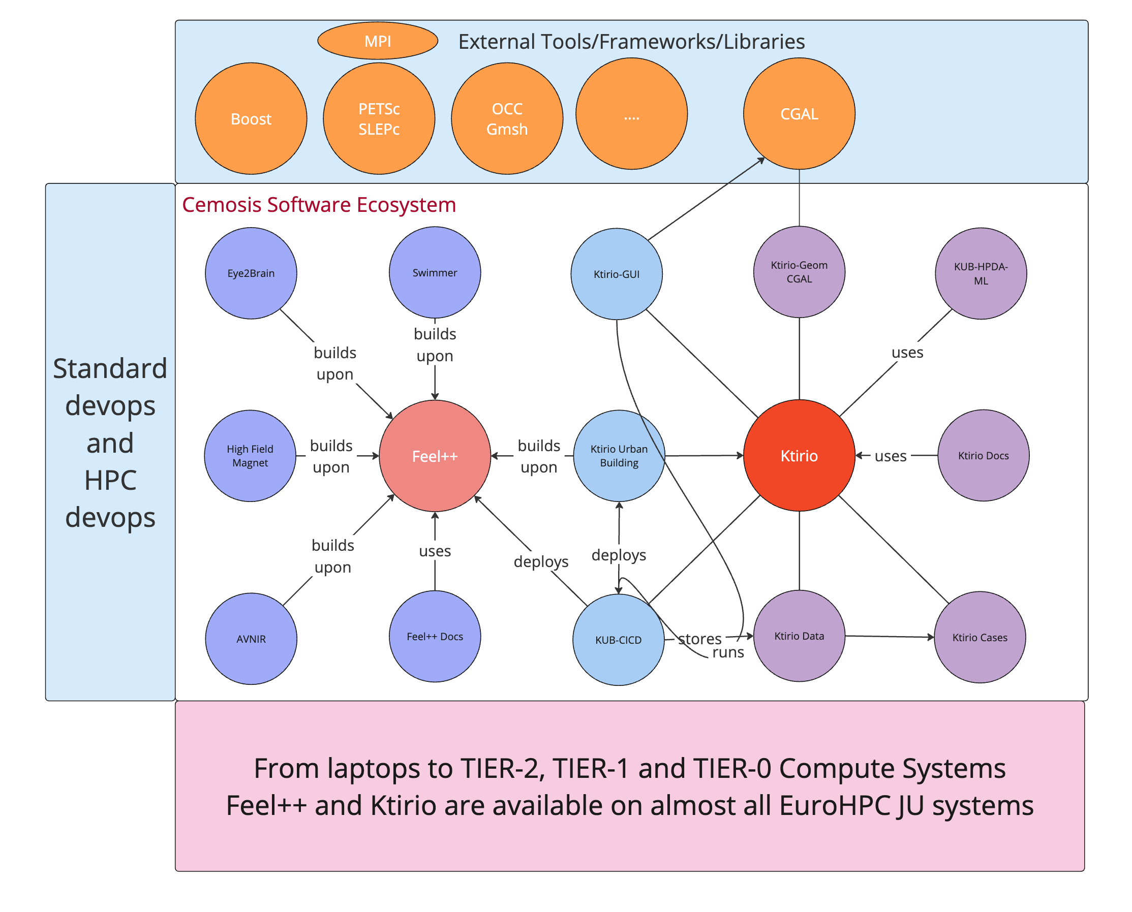
The Feel++ software

automation, code generation, applications

Christophe Prud'homme -- University of Strasbourg

Cemosis

What is Cemosis ?

Overview
  • Created in 2013, led by C Prud’homme

  • Hosted by IRMA (Institute for Advanced Mathematical Research) - Unistra

  • Organized in 3 poles :

  • Labeled Unistra platform in 2021 by the new Cortecs network (cortecs.unistra.fr)

  • Currently(2024/10) 7 engineers

Cemosis Software Eco-system

image

Our Current Big Projects

Feel++ Suite

What is Feel++ ?

Overview
  • Framework to solve problems based on ODE and PDE

  • C++17 and C++20

  • Python layer using Pybind11

  • Seamless parallelism with default communicator including ensemble runs

  • Powerful interpolation and integration operators working in parallel

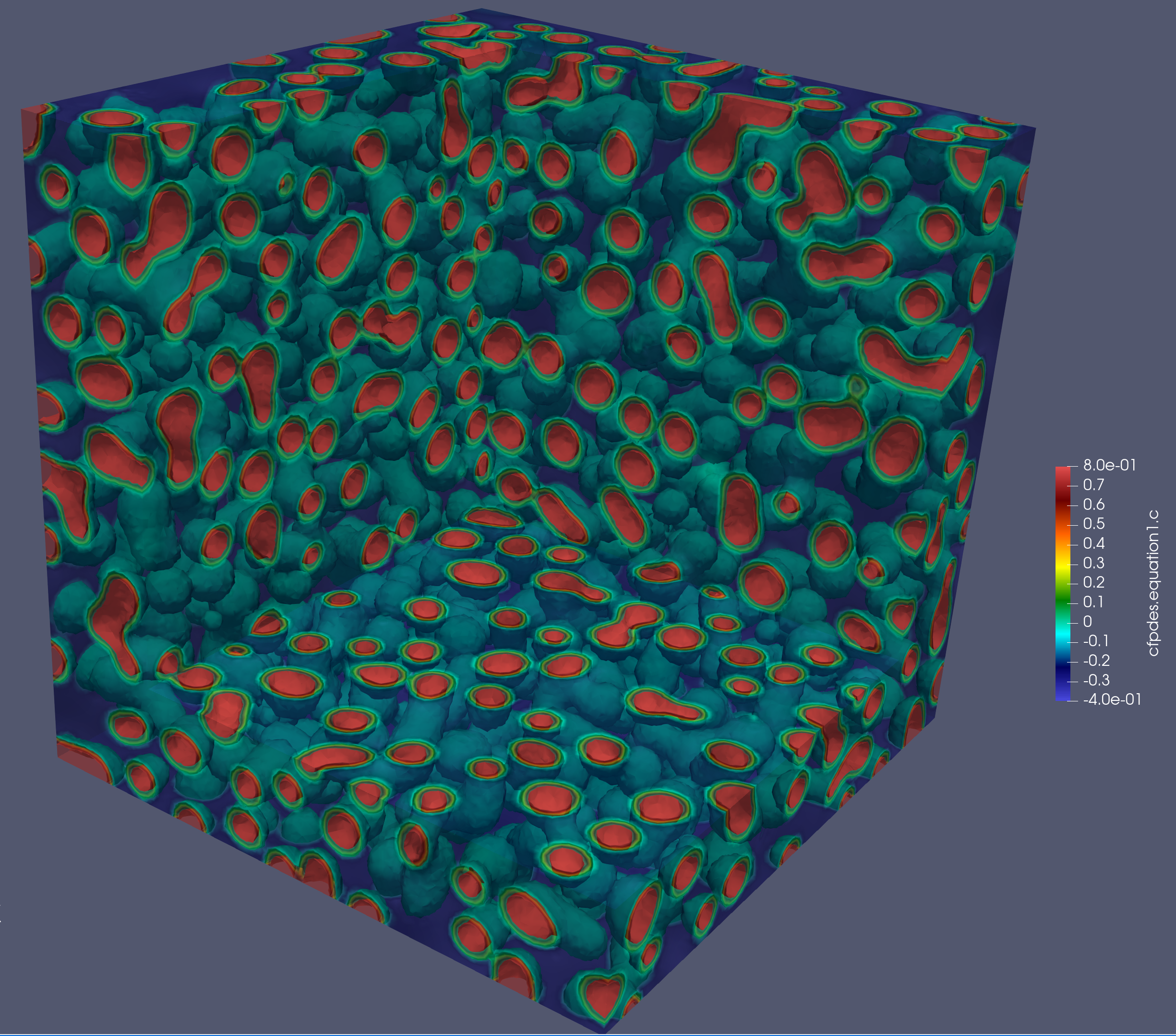
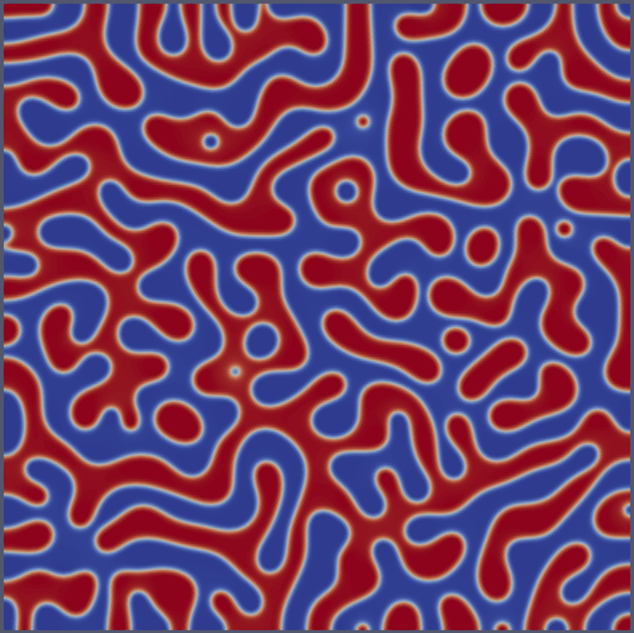
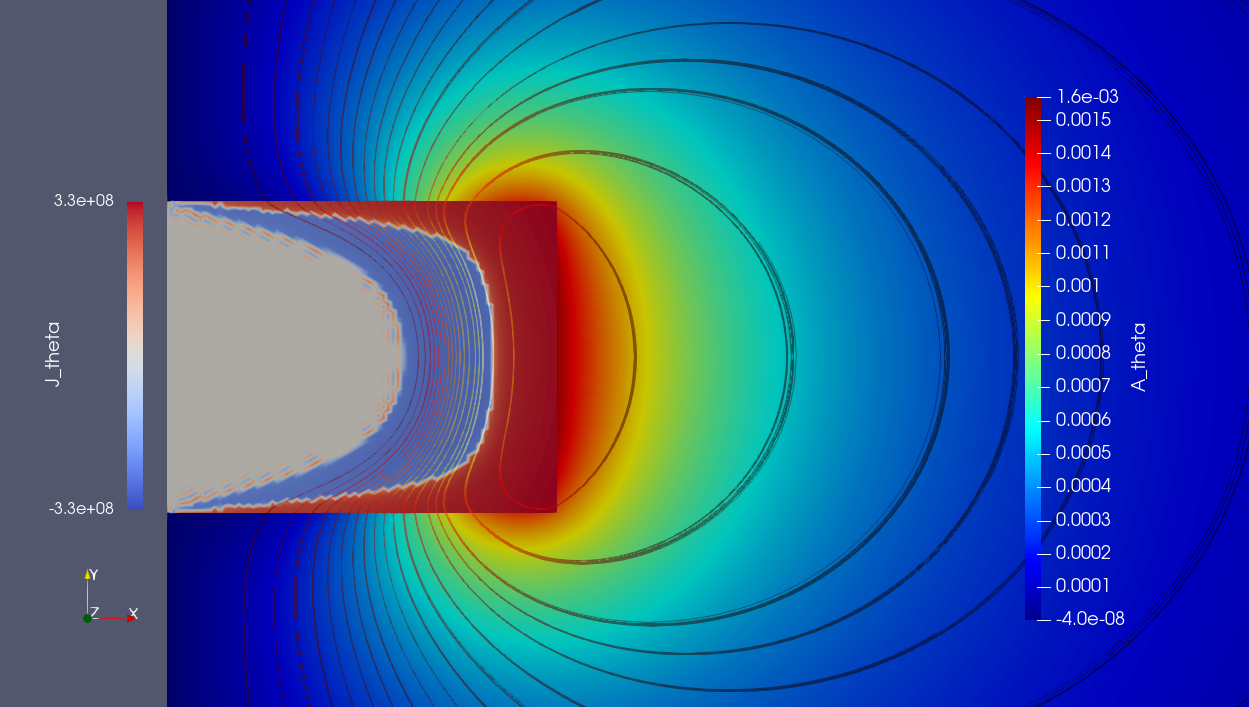
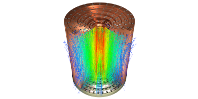
  • Advanced Post-processing including for high order approximation and high order geometry

  • Build: CMake and CMake Presets

  • Docs: https://docs.feelpp.org including dynamic pages that can be downloaded as notebooks
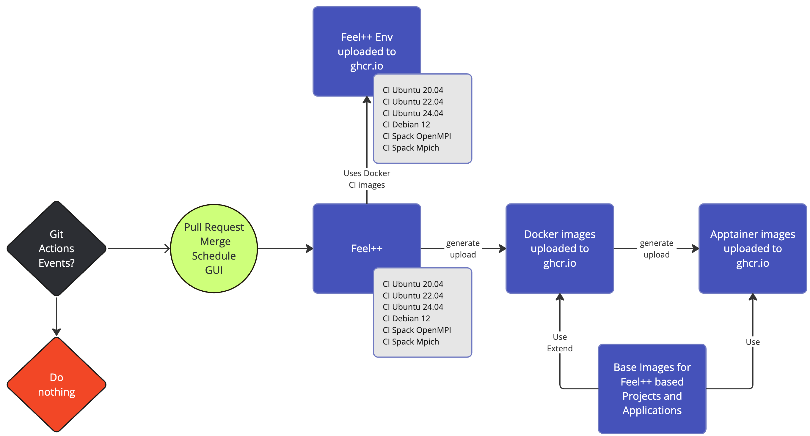
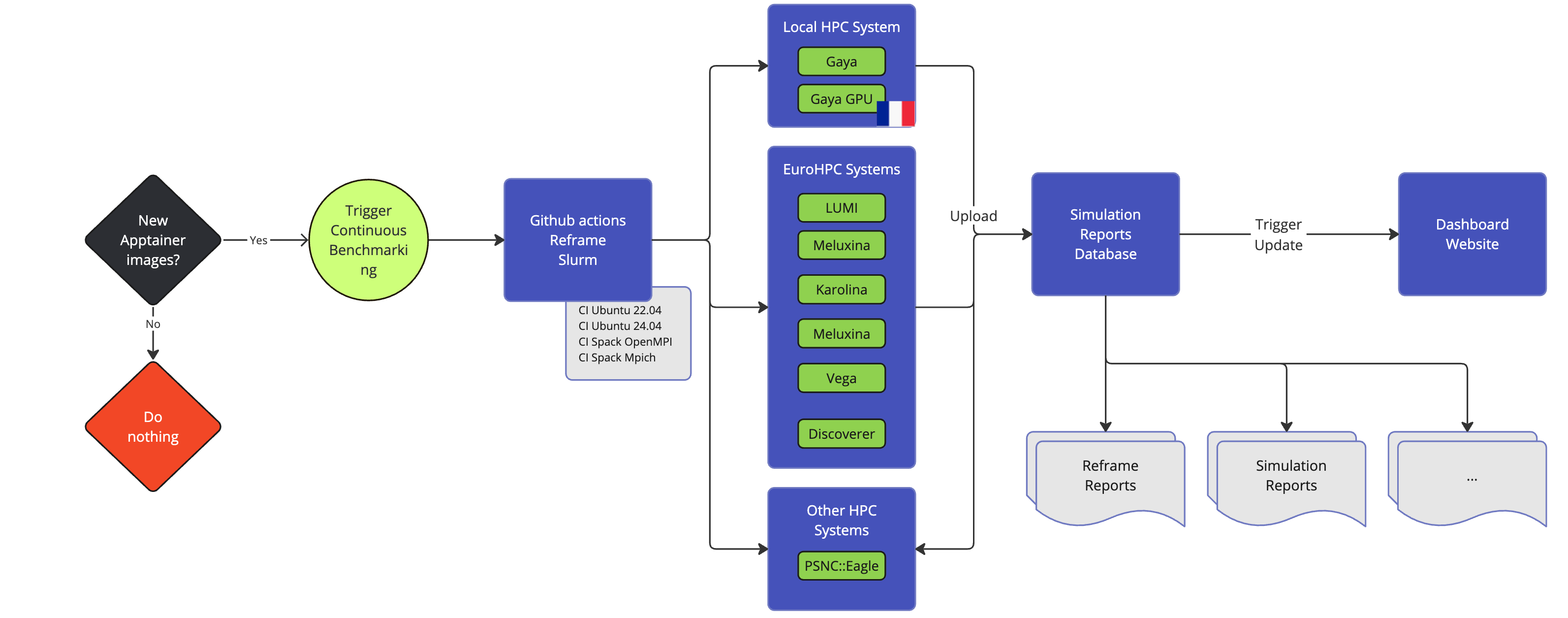
  • DevOps:

    • GitHub Actions: CI/CD and Continuous Benmarking on inHouse and EuroHPC systems

    • Packaging: Ubuntu/Debian, spack, MacPort

    • Containers: Docker, Apptainer

  • Tests: About a thousand tests in sequential and parallel C++ and Python

  • Usage: Research, R&D, Teaching, Services

image

Applications

Health(brain)

image

Health(Tumor cells)

image

Industry (ROM,UQ)

image

Health(Eye/Brain)

image

Health(Tomography)

image

Automotive(CFD,ROM)

image

Health(Rheology)

image

Physics(High Field Magnets)

image

Physics(Deflectometry)

image

Health(Micro swimmers)

image

Engineering (Buildings)

image

Health(Eye/Brain)

image

Feel++ Core Library

Laplacian
auto Vh = Pch<4>( mesh, markedelements(mesh, expr("<...>")) );
auto u = Vh->element(), v = Vh->element( g, "g" );
auto l = form1( _test = Vh );
l = integrate( _range = elements( support( Vh ) ),
               _expr = f * id( v ) );
l += integrate( _range = markedfaces( support( Vh ), "Robin" ), _expr = -r_2 * id( v ) );
l += integrate( _range = markedfaces( support( Vh ), "Neumann" ), _expr = -un * id( v ) );

auto a = form2( _trial = Vh, _test = Vh );
a = integrate( _range = elements( support( Vh ) ),
               _expr = inner( k * gradt( u ), grad( v ) ) );
a += integrate( _range = markedfaces( support( Vh ), "Robin" ), _expr = r_1*idt(u)*id(v));
a += on( _range = markedfaces( support(Vh), "Dirichlet" ), _rhs=l, _element=u, _expr = g );
a.solve( _rhs = l, _solution = u );
General Features
  • A large range of numerical methods to solve PDEs: cG, dG, hdG, rb/mor, …​

  • Finite Elements: \(L^2\), \(\mathbf{L}^2\), \(\mathbb{L}^2\), \(H^1\), \(\mathbf{H}^1\), \(\mathbb{H}^1\), \(\mathbf{H}(\text{div})\), \(\mathbf{H}(\text{curl})\), …​

  • Value types: single, double, double double, quad double, mp precision and complex…​

  • 0D+t, 1D(+t), 2D(+t), 3D(+t)

  • DSEL for Galerkin methods in C++

  • Linear algebra: PETSc/SLEPc, Eigen, Boost::ublas …​

Feel++ DSEL

Incompressoble Navier Stokes Equations
// test strain tensor
auto def = 0.5*(grad(v)  + trans(grad(v)));
// trial strain tensor
auto deft = 0.5*(gradt(u) + trans(gradt(u)));
// oseen
form2( _test=Xh, _trial=Xh, _matrix=M) =
  // automatic quadature
  integrate( elements(Xh->mesh()),
             alpha*trans(idt(u))*id(v)
             + 2.0*nu*trace(trans(deft)*def)
             + trans(gradt(u)*idv(beta))*id(v)
             - div(v)*idt(p) + divt(u)*id(q) );
General Features
  • Advanced DSEL

  • Automatic differentiation

  • Automatic quadrature

  • Automatic assembly

  • Automatic parallelism

Feel++ Continuous Integration/Delivery/Deployment

background

Feel++ Continuous Benchmarking

background

Feel++ Other features

Remeshing, distance to range, fast marching
// Named Arguments
auto Xh=Pch<1>(_mesh=mesh); (1)
auto u = Xh->element();
// expression handling
auto e3 = expr( "2*x*u*v:x:u:v" ); (2)
auto e3v = expr( e3, symbolExpr( "u", dxv( u ) ), symbolExpr( "v", Nx() ) );
// remeshing in seq and //
auto rm = remesh(_mesh=mesh,_params=<remeshing specs in json>); (3)
// Fast marching : compute distance to range
auto distToBoundary = distanceToRange( _space=Vh, _range=boundaryfaces( mesh ) ); (4)
auto distToBoundaryNarrowBand = (5)
   distanceToRange( _space=Vh, _range=boundaryfaces( mesh ),
                    _max_distance=3.*mesh->hAverage() );
1Expressivity: using our own named arguments library
2Expressions handling: based on Ginac, handles automatic differentiation, JIT compilation
3Remeshing in seq and parallel
4Versatile levelset/fast marching framework
5Narrow band FMM
Expression framework and Automatic differentiation
auto mesh = loadMesh<Mesh<Simplex<3,1>>();
auto Vh = Pch<2>( mesh ); (1)
auto u = Vh->element( inner(P()) ); (2)
auto e1 = expr( "u*u:u"); (3)
auto e2 = expr( "2*e1:e1");
auto e3base = expr( "3*e2:e2");
// handle composition
auto e3 = expr( e3base, symbolExpr("e1",e1), symbolExpr("e2",e2), symbolExpr("u",inner(P()) )); (4)
auto grad_e3 = grad<3>( e3 ); (5)
auto diff_e3_x_exact = 3*4*inner(P())*2*Px();
auto diff_e3_y_exact = 3*4*inner(P())*2*Py();
auto diff_e3_z_exact = 3*4*inner(P())*2*Pz();
auto grad_e3_exact = trans(vec(diff_e3_x_exact,diff_e3_y_exact,diff_e3_z_exact));
// compute error (machine error expected)
double error_grad_e3 = normL2(_range=elements(mesh),_expr= grad_e3 - grad_e3_exact ); (6)
1create \(P^2_{c,h}\)
2create an element of Vh such that \(u(x)=x^T x\)
3create expressions
4define symbols in expressions
5differentiate the expressions
6compute \(L^2\) error norm

Feel++ Recent Developments:: Python

Feel++ in Python
import feelpp
from feelpp.operators import *

mesh= feelpp.load(m, mesh_name, 0.1)
Xh = feelpp.functionSpace(mesh=mesh)
v=Xh.element()
v.on(range=feelpp.elements(mesh), expr=feelpp.expr("1"))
e_meas = mesh.measure()
M=mass(test=Xh,trial=Xh,range=feelpp.elements(mesh))
assert(abs(M.energy(v,v)-e_meas)<1e-10)
S=stiffness(test=Xh,trial=Xh,range=feelpp.elements(mesh))
assert(S.energy(v,v)<1e-10)
v.on(range=feelpp.elements(mesh), expr=feelpp.expr("x+y:x:y"))
assert(abs(S.energy(v,v)-2*e_meas)<1e-10)
Other Features
  • Parallel execution of toolboxes

    • Advanced multi-physics simulations

    • Advanced parametric studies including UQ

    • Reinforcement learning for micro-swimming

    • Ensemble Runs

    • Ensemble kalman filter in applications with sensors

Feel++ Toolboxes in Python
import feelpp.core as fppc
from feelpp.toolboxes.core import *
from feelpp.toolboxes.fluid import *
from feelpp.toolboxes.heat import *

def simulate(toolbox, export=True, buildModelAlgebraicFactory=True,data=None):
    toolbox.init(buildModelAlgebraicFactory)
    #toolbox.printAndSaveInfo()
    if toolbox.isStationary():
        toolbox.solve()
        if export:
            toolbox.exportResults()
    else:
        if not toolbox.doRestart():
            toolbox.exportResults(toolbox.timeInitial())
        toolbox.startTimeStep()
        while not toolbox.timeStepBase().isFinished():
            if feelpp.Environment.isMasterRank():
                print("time simulation: {}s/{}s with step: {}".format(toolbox.time(),toolbox.timeFinal(),toolbox.timeStep()))
            toolbox.solve()
            if export:
                toolbox.exportResults()
            toolbox.updateTimeStep()
    return not toolbox.checkResults()

ht = heat(dim=3,order=1)
ok=simulate(ht)
meas = ht.postProcessMeasures().values()
df=pd.DataFrame([meas])
# do something with the pandas dataframe
....

cfd=fluid(dim=3,order=2)
ok=simulate(cfd)
....

Toolboxes

CFD

Features
  • Navier-Stokes incompressible 2D, 3D

  • Newtonian and non-newtonian

  • Multi-fluid support(levelset)

  • Moving domain support(ale)

  • Rigid and elastic body interaction.

  • Pressure BC.

  • Robust stab. methods.

  • WIP Turbulence Model.

  • Various formulations (e.g. Conservative, Curl, EMAC,…​)

CSM

  • Linear elasticity

  • Large deformations, large displacements (Hyper elasticity)

  • Compressible, nearly incompressible materials

  • Multi-material support

Heat Transfer

  • 2D and 3D heat transfer

  • High order in space and time

  • Diffusion and Convection

  • Robust Stab. Method

  • Thermo-Electric models including Seebeck/Peltier

  • Conjuguate heat transfer

  • RHT: on-going

Generic Toolbox :: Coefficient Form PDEs

Find scalar or vector fields \(u_i,i=1...,N\) such that

\[\begin{aligned} d_i \frac{\partial u_i}{\partial t} + \nabla \cdot \left( -c_i \nabla u_i - \alpha u_i + \gamma_i \right)& \\ + \beta_i \cdot \nabla u_i + a u_i &= f \quad \text{ in } \Omega \end{aligned}\]
  • Coefficients can depend on the unknowns \(u_j,j=1 \ldots N\).

  • Automatic differentiation built on top of Feel++ expression handling

  • Various schemes based on Newton or Picard

Predator-Prey coupled model [Github]
"Models": {
    "cfpdes":{ "equations":["equation1","equation2"] },
    "equation1":{
        "setup":{
            "unknown":{"basis":"Pch1","name":"prey","symbol":"u"},
            "coefficients":{
                "c":"1", // diffusion
                "a":"-( (1-equation1_u) - equation2_v/(equation1_u+thealpha) ):thealpha:equation1_u:equation2_v", // life and death
                "d":"1" // time derivative
            } } },
    "equation2":{
        "setup":{
            "unknown":{ "basis":"Pch1", "name":"predator", "symbol":"v" },
            "coefficients":{
                "c":"thedelta:thedelta", // diffusion
                "a":"-( (thebeta*equation1_u)/(equation1_u+thealpha) - thegamma ):thebeta:thealpha:thegamma:equation1_u", // life and death
                "d":"1"// time derivative
            } } } }
    ...

Cahn Hilliard

Cahn-Hilliard in L-Shape domain \(6e-3s\)

image ch2d

\[\begin{aligned} f(u)=u^2(u^2-1),\, \lambda=10^{-4} \end{aligned}\]
Phase separation modeling
\[\begin{aligned} \partial_t u-\nabla \cdot M\left(\nabla\left(f'(u)-\lambda \Delta u\right)\right)&=0 \quad \text { in } \Omega \text {, }\\ M\nabla\left(f'(u)-\lambda \Delta u\right)&=0 \text { on } \partial \Omega,\\ M \lambda \nabla u \cdot n&=0 \quad \text { on } \partial \Omega . \end{aligned}\]
Mixed Form
\[\begin{array}{rl} \frac{\partial u}{\partial t}-\nabla \cdot M \nabla \mu &=0 \quad \text { in } \Omega, \\ \mu-f'(u)+\lambda \Delta u&=0 \text { in } \Omega . \end{array}\]
2D
3D
Phase separation modeling
"Models":
{
  "cfpdes":{ "equations":["equation1","equation2"] },
  "equation1":{
    "setup":{
        "unknown":{"basis":"Pch1","name":"c","symbol":"c"},
        "coefficients":{
           "d": "1",
           "gamma": "{-equation2_grad_mu_0,-equation2_grad_mu_1,-equation2_grad_mu_2}"
  }}},
  "equation2":{
    "setup":{
        "unknown":{"basis":"Pch1","name":"mu","symbol":"mu"},
        "coefficients":{
           "gamma":"{lambda*equation1_grad_c_0,lambda*equation1_grad_c_1, lambda*equation1_grad_c_2}",
           "a":"1",
           "f": "equation1_c^2*(equation1_c^2 - 1)"
  } } }
}
Model equations
\[\begin{aligned} -\frac{1}{\mu}\Delta a_\theta + \frac{1}{\mu r^2}a_\theta + \sigma \frac{\partial a_\theta}{\partial t} =0 &\text{ in } \Omega \\ a_\theta = \frac{r}{2}\text{B}_\text{applied} &\text{ on } \partial\Omega \end{aligned}\]
Non-Linear Part (e-j power law):
\[\sigma=\begin{cases}\frac{j_c}{e_c}\left(\frac{||-\partial a_\theta / \partial t||}{e_c}\right)^{(1-n)/n} &\text{in Superconductor}\\ 0 &\text{in Air} \end{cases}\]

feelpp example supra

Bulk Superconductor Model
"Models":{
    "cfpdes":{ "equations":"magnetic" },
    "magnetic":{
        "common":{"setup":{"unknown":{
            "basis":"Pch1",
            "name":"Atheta","
            symbol":"Atheta"
        }}},
        "models":[{
            "name":"magnetic_Conductor",
            "materials":"Conductor",
            "setup":{"coefficients":{
                    "c":"x/mu:x:mu",
                    "a":"1/mu/x:mu:x",
                    "d":"materials_Conductor_sigma*x
                         :materials_Conductor_sigma:x"}}
        },{
            "name":"magnetic_Air",
            "materials":"Air",
            "setup":{"coefficients":{
                    "c":"x/mu:x:mu",
                    "a":"1/mu/x:mu:x"}}}
        ]
    }
}
...

Toolbox:: Hybridized Discontinuous Galerkin

Second order elliptic problems

Darcy
\[\begin{aligned} \mathbf{j} + \mathbf{K} \nabla p &= 0 & \text{ in } \Omega \\ \nabla \cdot \mathbf{j} &= f & \text{ in } \Omega \\ p &= 0 & \text{ on } \Gamma_D \\ \mathbf{j} \cdot \mathbf{n} &= g_N & \text{ on } \Gamma_N \end{aligned}\]
  • \(p\) is the potential

  • \(\mathbf{j}\) is the flux

Elasticity, \(d=2,3\)
\[\begin{aligned} \mathbf{A} \underline{\boldsymbol{\sigma}}-\underline{\boldsymbol{\epsilon}}(\boldsymbol{u})&=0 \quad \text { in } \Omega \subset \mathbb{R}^{d},\\ \nabla \cdot \underline{\boldsymbol{\sigma}}&=\boldsymbol{f} \quad \text { in } \Omega,\\ \boldsymbol{u}&=\boldsymbol{g} \text { on } \partial \Omega . \end{aligned}\]
  • \(\boldsymbol{u}: \Omega \rightarrow \mathbb{R}^{3}\) displacement

  • \(\underline{\boldsymbol{\epsilon}}(\boldsymbol{u}):=\frac{1}{2}\left(\nabla \boldsymbol{u}+(\nabla \boldsymbol{u})^{\top}\right)\) strain tensor

  • \(\underline{\boldsymbol{\sigma}}: \Omega \rightarrow S\) stress tensor where \(S\) is the set of all symmetric matrices in \(\mathbb{R}^{d\times d}\)

Methodology: HDG

  • Provides optimal approximation of both primal and flux/stress variables \(p/\boldsymbol{u}\) and \(\mathbf{j}/\underline{\boldsymbol{\sigma}}\) respectively;

  • Requires less globally coupled degrees of freedom than DG methods of comparable accuracy;

  • Allows local element-by-element postprocessing to obtain new approximations with enhanced accuracy and conservation properties

Some Applications

  • Electrostatic

  • Heat transfer

  • Flow in porous media

  • Elasticity and Poro-Elasticity

The integral boundary condition

Electric potential in a nanoscale floating gate nMOS

image

Magnetic field in a high field magnet (\(36T\))

image

Tissue perfusion in the Lamina Cribrosa

image

Feature: Integral Boundary Condition (IBC)
\[\begin{aligned} \int_{\Gamma_{ibc}} \mathbf{j} \cdot \mathbf{n} &= I_{target}\\ p&=\text{constant but unknown} \end{aligned}\]
  • A HDG method for elliptic problems with integral boundary condition: Theory and Applications, Silvia Bertoluzza,Giovanna Guidoboni,Romain Hild,Daniele Prada,Christophe Prud’homme,Riccardo Sacco,Lorenzo Sala,Marcela Szopos, 2021 submitted

HDG Laplacian: formulation

Notations
  • \(\mathbf{T}_h\) the collection of elements \(K\) such that \(\Omega = \bigcup_{K\in \mathbf{T}_h} K\).

  • \(h:= max_{K \in \mathbf{T}_h} h_K\), \(\partial K\) the boundary of \(K\) with its measure \(|F|\)

  • \(\mathbf{n}_{\partial K}\) is the associated unit outward normal vector.

  • The skeleton of \(\mathbf{T}_h\) is the collection of all the faces of \(\mathbf{T}_h\) into the set \(\mathbf{F}_h\).

  • \(\mathbf{F}_h = \mathbf{F}_h^\Gamma \cup \mathbf{F}_h^0, \; \mathbf{F}_h^\Gamma = \mathbf{F}_h^D \cup \mathbf{F}_h^N \cup \mathbf{F}_h^{ibc}\)

Function Spaces
  • \(V_h = \Pi_{K \in \mathbf{T}_h} V(K), \qquad V(K) = \left[ P_k (K) \right]^n\)

  • \(W_h = \Pi_{K\in\mathbf{T}_h} W(K), \qquad W(K) = \left[ P_k (K) \right]\)

  • \(\widetilde M_h = \{ \mu \in L^2(\mathbf{F}_h): \mu\rvert_F \in P_k(F) \; \forall F \in \mathbf{F}_h \setminus \mathbf{F}_h^{ibc} \},\)

  • \(M^*_h = \{ \mu \in C^0(\mathbf{F}^{ibc}_h): \mu\rvert_F \in P_0(F) \; \forall F \in \mathbf{F}_h^{ibc} \} \cong \mathbb{R}\)

  • \(M_h=\widetilde M_h \oplus M^*_h\)

HDG Laplacian: formulation

Discrete formulation Find \(\boldsymbol{j}_h \in V_h, \; p_h \in W_h\) and \(\hat{p}_h \in M_h\) such that:

\[\begin{aligned} \sum_{K\in\mathbf{T}_h} \left[ \left( \mathbf{K}^{-1} \boldsymbol{j}^K_h, \boldsymbol{v}_h^K \right)_K - \left( p_h^K, \nabla\cdot\boldsymbol{v}_h^K \right)_K + \langle \hat{p}_h, \boldsymbol{v}_h^K \cdot {\boldsymbol{n}}_{\partial K}\rangle_{\partial K} \right] = 0 && \forall \boldsymbol{v}_h \in V_h \\ \sum_{K\in\mathbf{T}_h} \left[ -\left(\boldsymbol{j}_h^K,\nabla w_h^K \right)_K + \langle \hat{\boldsymbol{j}}_h^{\partial K}\cdot {\boldsymbol{n}}_{\partial K}, w_k^K \rangle_{\partial K} \right] = \sum_{K\in\mathbf{T}_h} \left( f, w_h^K \right)_K && \forall w_h \in W_h \\ \sum_{K\in\mathbf{T}_h} \langle \hat{\boldsymbol{j}}_h^{\partial K} \cdot {\boldsymbol{n}}_{\partial K}, \mu_h \rangle_{\partial K} = \langle g_N, \mu_h \rangle_{\Gamma_N} + I_{target} |\Gamma_{ibc}|^{-1} \langle\mu_h, 1\rangle_{\Gamma_{ibc}} && \forall \mu_h \in M_h\\ \hat{\mathbf j}_h^{\partial K} = \mathbf j_h^K + \tau_K(p_h^K - \hat{p_h}^{\partial K})\mathbf n && \forall\partial K, \end{aligned}\]

HDG Laplacian

Meshes
auto mesh=loadMesh(_mesh=new Mesh<Simplex<3>>); (1)
auto complement_integral_bdy = complement(faces(mesh), (2)
  [&mesh]( auto const& e ) {
    if ( e.hasMarker() &&
         e.marker().matches(mesh->markerName("Ibc*") ) )
      return true;
    return false;
   });
auto face_mesh = createSubmesh( mesh, complement_integral_bdy); (3)
auto ibc_mesh = createSubmesh( mesh, markedfaces(mesh,"Ibc*")); (4)
1load mesh
2build set of non ibc facets
3\(\mathbf{F}_h^{ibc}\) and
4\(\mathbf{F}_h\setminus\mathbf{F}_h^{ibc}\).
Function Spaces
Vh_ptr_t Vh = Pdhv<OrderP>( mesh); (1)
Wh_ptr_t Wh = Pdh<OrderP>( mesh );
Mh_ptr_t Mh = Pdh<OrderP>( face_mesh );
// only one degree of freedom
Ch_ptr_t Ch = Pch<0>(ibc_mesh );
// $n$ IBC
auto ibcSpaces = product( nb_ibc, Ch); (2)
auto Xh = product( Vh, Wh, Mh. ibcSpaces  ); (3)
1create the spaces \(V_h,W_h,\tilde{M}_h\) and \(M_h^*\).
2handle arbirary number of IBCs
3initialize spaces and product space
\[V_h\times W_h\times \tilde{M}_h\times (M_h^*)^n\]

HDG laplacian

Construction of algebraic system
auto a = blockform2( Xh )
auto rhs = blockform1( Xh );

. . .
// Assembling the right hand side
rhs(1_c) += integrate(_range=elements(mesh),_expr=-f*id(w));
. . .
// Assembling the main matrix
a(0_c,0_c) += integrate(_range=elements(mesh),
                        _expr=(trans(lambda*idt(u))*id(v)) );
. . .
//$\langle \hat{p}_h\rvert_{\tilde{M}_h}, \boldsymbol{v}_h^K \cdot {\boldsymbol{n}}_{\partial K}\rangle$ $$
a(0_c,2_c) += integrate(_range=internalfaces(mesh),
         _expr=( idt(phat)*(leftface(trans(id(v))*N())+
                rightface(trans(id(v))*N()))));
solving and postprocessing
a( 3_c, 0_c, i, 0 ) +=
   integrate( _range=markedfaces(mesh,"Ibc"),
             _expr=(trans(idt(u))*N()) * id(nu) );
auto U = Xh.element();
a.solve(_solution=U, _rhs=rhs, _name="hdg");
auto up = U(0_c);
auto pp = U(1_c);
auto phat = U(2_c);
auto ip = U(3_c,0);

// postprocessing
auto Whp = Pdh<OrderP+1>( mesh );
auto pps = product( Whp );
auto PP = pps.element();
auto ppp = PP(0_c);
auto b = blockform2( pps, solve::strategy::local, backend() );
b( 0_c, 0_c ) = integrate( _range=elements(mesh), _expr=inner(gradt(ppp),grad(ppp)));
auto ell = blockform1( pps, solve::strategy::local, backend() );
ell(0_c) = integrate( _range=elements(mesh), _expr=-lambda*grad(ppp)*idv(up));
b.solve( _solution=PP, _rhs=ell, _name="sc.post", _local=true);
ppp=PP(0_c);
ppp += -ppp.ewiseMean(P0dh)+pp.ewiseMean(P0dh);

Toolbox HDG

  • Similar to CFPDEs, except that only one equation for now

    • time dependence

    • Other terms in the PDEs

    • non-linear coefficients

  • IBCs

    • arbitrary number

    • Coupling with 0D+t models using FMU

      • time splitting approach to avoid iterating

  • Extended to PoroElasticity

  • WIP: HHO support

  • WIP: Order reduction (RB and NiRB)

  • Future: merge with CFPDEs

High Field Magnets resistive / superconductors magnets

image

Ocular Mathematical Virtual Simulator (OMVS)

image

Final Words

  • Develop Feel++ as a service

  • Streamline complex workflows for advanced usage/studies

    • data assimilation,

    • machine learning (interface with Scimba and Scikit-learn),

    • UQ on complex models (interface with OpenTURNs)

    • …​

  • Go Digital twins

    • Building energy modeling (Ktirio Urban Building - CoE Hidalgo2)

    • High field magnets (LNCMI)

    • Eye (Eye2Brain)